Big O is a fundamental concept in the field of computer science, but most people do not understand what it is and why it is necessary. It is also very difficult to grasp for beginners. In this article, we will demystify Big O, understand its importance, and explore how it can be used to determine the efficiency of algorithms.

Prerequisite

• Basic understanding of data structures like arrays.

• Basic knowledge of JavaScript(our examples are in javascript syntax)

What is Big O?

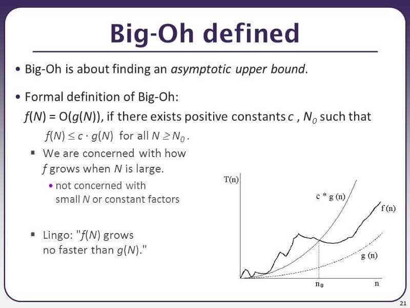
This image above explains Big O as 'finding an asymptotic upper bound', but that's not why we're here, we came for a more simplistic explanation, not this one 😂😂😂😂. So let's define it then.

Big O is a way to express and represent an algorithm's performance. An algorithm is a step-by-step approach to solving problems, and it is important to know that a problem can have multiple algorithms for finding its solution, the Big O notation is a standard for identifying the most optimal/effective algorithm.

Big O measures an algorithm's performance in terms of two factors which are, the amount of time it takes to complete and the amount of memory it consumes. This being said, there are two ways to measure the performance of any algorithm using Big O;

• Time complexity.
• Space complexity.

Time complexity

Time complexity is how quickly an algorithm accomplishes its objective. Basically, it is how long an algorithm will take to accomplish its goal, and it is determined by how well it performs as the number of operations increases.

Space complexity

This is how much memory an algorithm consumes in performing its required task. An algorithm's space complexity is determined by the amount of memory space necessary to solve an instance of the computational problem.

Importance of Big O

A major significance of Big O is that it serves as a standard for the comparison of algorithms. As we stated earlier, several algorithms can be used to solve a single problem, and Big O is a way to determine the most efficient algorithm for solving that problem.

Other objectives of Big O include the following;

• Determining an algorithm's worst-case running time based on the size of its input.

• Analysing algorithms in terms of scalability and efficiency.

Types Of Big O notations

There are several Big O Notations but before we dive into them let's analyze the image below.

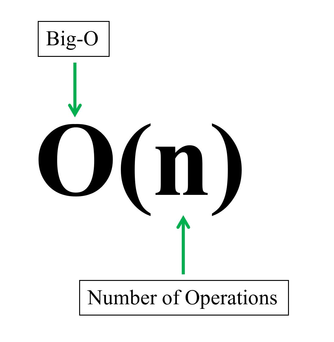
This image is a format used for representing Big O notations and it can be broken down into the following two parts.

• O, which stands for Big O
• n, which stands for the number of operations.

Note: The number of operations represents the number of tasks/activities the algorithm handles.

With the aid of the diagram below, we will discuss the types of Big O notations while focusing on the best three(3) notations.

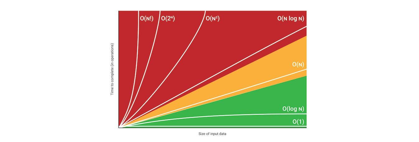
The image above is a graph showing several Big O notations and the colors represent the following;

• The red 🟥 region, represents the worst-case scenario of any algorithm. In this region, we have the O(N!), O(N²), O(2ⁿ), and O(N log N) notations.

• The yellow 🟨 region, represents an intermediate-level scenario of any algorithm. Any algorithm in this region is suitable and okay, compared to those in the red region. It consists of the O(N) notation.

• The green 🟩 region, represents the best-case scenario of any algorithm. This is the desired state of every algorithm and it consists of the O(1) and O(log N) notations.

Let's now dive deep into the yellow and green regions, which consist of the following notations;

• O(1) - constant complexity
• O(N) - Linear complexity
• O(Log N) - logarithmic complexity

O(1)- Constant complexity

Constant-time algorithms follow O(1) notation, which means that their time complexity is constant. Regardless of the amount of input they receive, constant-time algorithms run in the same amount of time.

Thus, if you are given;

• 1 input, it will run in 1 second

• 10 inputs, it will run in 1 second

• 100, 000 inputs, it will run in 1 second.

Let's take a code example.

const example1 = function (names) {
  console.log(names[0]);
};

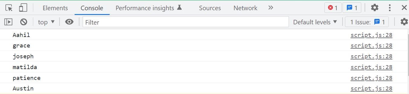
example1(["Aahil", "grace", "joseph", "matilda", "patience", "Austin"]);

In the example above, we created a function called example1 which takes an array of names as input. The function is simply made to carry out one (1) activity, which is to print to the browser's console, the first name in the array.

Output 👇

This example above has a constant time complexity and we can say that it performs a constant number of operations regardless of inputs. That is to say, even if we were to find the third and last names of the array, it would still have a constant time because it is still carrying out the same operation of finding a name from the array.

Note: O(1) is the best-case scenario of any algorithm.

O(N) - Linear complexity

An algorithm with a notation of O(N) scales as input scales between the number of inputs and the number of operations. As the input increases, the algorithms take a proportionately longer time to complete.

Therefore, if you are given;

• 1 input, it will carry out 1 operation.

• 10 inputs, will carry out 10 operations.

• 100, 000 inputs, will carry out 100, 000 operations.

It has a linear performance either in time or space complexity. As the number of inputs increases, the number of operations increases, and the amount of time it takes to complete increases also.

For instance, when reading a book, it takes more time to finish depending on how many pages that book has. Therefore, it'll take a shorter time to read a book of 10 pages, than a book of 1000 pages. This is a more relatable example, now let's take a practical code example.

const example2 = function (names) {
  for (const name of names) console.log(name);
};

example2(["Aahil", "grace", "joseph", "matilda", "patience", "Austin"]);

In our example above, we created a function called example2 which takes the array of names as input. The function contains a for...of loop, which loops through the array of names and prints each name in the array to the console. The function is called with an array of 6 names.

Output 👇

In this example, if more names were added to the array, it would take a longer time to complete, therefore we can say that it has linear time complexity.

In terms of space complexity, we created just one variable, but that variable will occupy space that is equivalent to storing all the names in the array. Therefore, as the names in the array increase, the size of the variable increases as well.

O(Log N) - logarithmic complexity

In an algorithm whose complexity is O(log N), the number of operations increases very slowly with increasing input sizes. As input size grows exponentially, the calculation time barely increases.

Therefore, if you are given;

• 1 input, it will run in 1 second

• 10 inputs, it will run in 2 seconds.

• 100 inputs, it will run in 3 seconds.

Note: The following are a few things to note about O(log N);

• An example of O(log N) is the binary search.
• It is far more performant that an algorithm with O(N).

Below is a summary table that explains the nature of most of the Big O notations

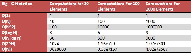
In the table above we can see that notations in the red region such as O(N!) are unoptimized and they produce very large complexities in terms of space and time regardless of the number of inputs. Algorithms with notations in the red region take a longer time to finish when given large inputs and they would take up a lot of space/memory. Therefore, it is advised that algorithms with such notations be optimized or disregarded when solving problems.

It is also noteworthy that O(1) is the best performance an algorithm can have. Most algorithms can be optimized to get to the yellow or green region of the previous chart i.e., O(1), O(log N), and O(N) depending on certain tradeoffs.

Conclusion

As we have come to the conclusion of this article, and hopefully we were able to accomplish all the objectives we set at the beginning, I would like to conclude that Big-O notation indicates how well algorithms perform on large problems, such as sorting or searching large lists.